Load Mass Spectrum and calculate metrics
import natorgms.draw as draw
from natorgms.spectrum import Spectrum

import pandas as pd
import numpy as np
import matplotlib.pyplot as plt
Load and save
Load mass spectrum from csv file. When loading, if the headings of m/z and intensity are not default (“mass”, “intensity”), you must specify them by mapper. You also need to specify a separator (default is “,”). In order not to load unnecessary data, we will also set the take_only_mz flag True.
spec = Spectrum.read_csv(filename = "data/sample2.csv",
                            mapper = {'m/z':'mass', "I":'intensity'},
                            take_only_mz = True,
                            sep = ',',
                            )
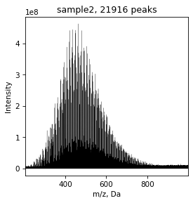
Now we can plot spectrum
draw.spectrum(spec)
The next step is assignement of brutto formulas for the masses. By default, this process is performed on the following range of elements: ‘C’ from 4 to 50, ‘H’ from 4 to 100, ‘O’ from 0 to 25, ‘N’ from 0 to 3, ‘S’ from 0 to 2. The following rules are also followed by default: 0.25<H/C<2.2, O/C < 1, nitogen parity, DBE-O <= 10.
We can specify elements by brutto_dict parameters as bellow. If you want use isotopes use “_” and number, for example “C_13”
rel_error is allowable relative error. By default it is 0.5
spec = spec.assign(brutto_dict={'C':(4,51), 'C_13':(0,3), 'H':(4,101), 'O':(0, 26), 'N':(0,3)}, rel_error=0.5)
Now you can see masses with brutto formulas. But first we can drop unassigned formulas
spec = spec.drop_unassigned()
spec.table
| mass | intensity | assign | C | C_13 | H | O | N | |
|---|---|---|---|---|---|---|---|---|
| 0 | 205.08706 | 5072918 | True | 12.0 | 0.0 | 14.0 | 3.0 | 0.0 |
| 1 | 207.06445 | 3388781 | True | 13.0 | 1.0 | 9.0 | 1.0 | 1.0 |
| 2 | 209.04557 | 6721187 | True | 10.0 | 0.0 | 10.0 | 5.0 | 0.0 |
| 3 | 209.08202 | 4015701 | True | 11.0 | 0.0 | 14.0 | 4.0 | 0.0 |
| 4 | 210.02769 | 3463522 | True | 12.0 | 1.0 | 6.0 | 3.0 | 0.0 |
| ... | ... | ... | ... | ... | ... | ... | ... | ... |
| 6273 | 991.68139 | 8570909 | True | 46.0 | 2.0 | 98.0 | 18.0 | 2.0 |
| 6274 | 993.51449 | 10621638 | True | 41.0 | 2.0 | 80.0 | 23.0 | 2.0 |
| 6275 | 993.71227 | 8240803 | True | 50.0 | 2.0 | 100.0 | 15.0 | 2.0 |
| 6276 | 995.67950 | 9630054 | True | 50.0 | 2.0 | 98.0 | 17.0 | 0.0 |
| 6277 | 999.37335 | 8356890 | True | 43.0 | 2.0 | 62.0 | 23.0 | 2.0 |
6278 rows × 8 columns
After assignment we can calculate different metrics: H/C, O/C, CRAM, NOSC, AI, DBE and other. We can do it separate by such methods as calc_ai, calc_dbe … or do all by one command calc_all_metrics
spec = spec.calc_all_metrics()
Now we can see all metrics
spec.table.columns
Index(['mass', 'intensity', 'assign', 'C', 'C_13', 'H', 'O', 'N', 'calc_mass',
       'abs_error', 'rel_error', 'DBE', 'DBE-O', 'DBE_AI', 'CAI', 'AI',
       'DBE-OC', 'H/C', 'O/C', 'class', 'CRAM', 'NOSC', 'brutto', 'Ke', 'KMD'],
      dtype='object')
You can save the data with spectrum and calculated metrics to a csv file at any time by to_csv method
spec.to_csv('temp.csv')
Draw
Data can be visualized by different methods
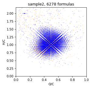
Simple Van-Krevelen diagramm. By default CHO formulas is blue, CHON is orange, CHOS is green, CHONS is red. There is no S, so it is only two colors here
draw.vk(spec)
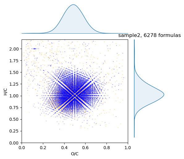
We can plot it with density axis
draw.vk(spec, draw.scatter_density)
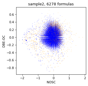
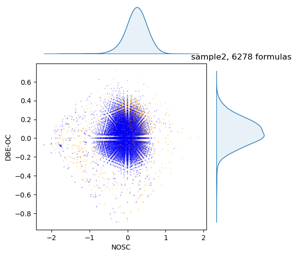
Or do it with any of metrics in spectrum. For example, NOSC vs DBE-OC
draw.scatter(spec, x='NOSC', y='DBE-OC')
draw.scatter_density(spec, x='NOSC', y='DBE-OC')
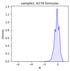
We can plot separate density
draw.density(spec, 'AI')
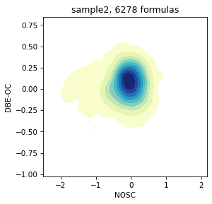
Or plot 2D kernel density scatter
draw.density_2D(spec, x='NOSC', y='DBE-OC')
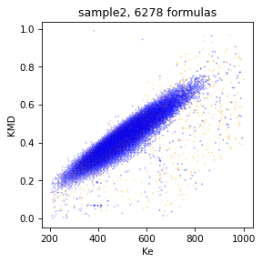
We can plot Kendric diagramm by command
draw.scatter(spec, x='Ke', y='KMD')
Molecular class
We can get average density of molecular classes of brutto formulas in spectrum
spec.get_mol_class()
| class | density | |
|---|---|---|
| 0 | unsat_lowOC | 0.553290 |
| 1 | unsat_highOC | 0.404771 |
| 2 | condensed_lowOC | 0.000409 |
| 3 | condensed_highOC | 0.000278 |
| 4 | aromatic_lowOC | 0.010322 |
| 5 | aromatic_highOC | 0.000261 |
| 6 | aliphatics | 0.008320 |
| 7 | lipids | 0.003229 |
| 8 | N-satureted | 0.009970 |
| 9 | undefinded | 0.009150 |
Metrics
We can get any metrics that avarage by weight of intensity.
spec.get_mol_metrics()
| metric | value | |
|---|---|---|
| 0 | AI | -0.016670 |
| 1 | C | 24.216486 |
| 2 | CAI | 12.502903 |
| 3 | CRAM | 0.798058 |
| 4 | C_13 | 0.231241 |
| 5 | DBE | 12.569666 |
| 6 | DBE-O | 0.742390 |
| 7 | DBE-OC | 0.027562 |
| 8 | DBE_AI | 0.624843 |
| 9 | H | 25.873668 |
| 10 | H/C | 1.057624 |
| 11 | N | 0.117547 |
| 12 | NOSC | -0.064638 |
| 13 | O | 11.827276 |
| 14 | O/C | 0.489112 |
| 15 | mass | 509.495873 |
spec.get_mol_metrics(metrics=['AI', 'DBE', 'NOSC', 'H/C', 'O/C'])
| metric | value | |
|---|---|---|
| 0 | AI | -0.016670 |
| 1 | DBE | 12.569666 |
| 2 | H/C | 1.057624 |
| 3 | NOSC | -0.064638 |
| 4 | O/C | 0.489112 |
We can avarage the same by mean or other function(max, min, std, median)
spec.get_mol_metrics(metrics=['AI', 'DBE', 'NOSC', 'H/C', 'O/C'], func='mean')
| metric | value | |
|---|---|---|
| 0 | AI | -0.099484 |
| 1 | DBE | 12.824626 |
| 2 | H/C | 1.088260 |
| 3 | NOSC | -0.117060 |
| 4 | O/C | 0.462034 |
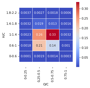
Also we can split VanKrevelen diagramm to squares and calculate density in each squares
spec.get_squares_vk(draw=True)
| value | square | |
|---|---|---|
| 0 | 0.000059 | 1 |
| 1 | 0.001766 | 2 |
| 2 | 0.002253 | 3 |
| 3 | 0.003180 | 4 |
| 4 | 0.003691 | 5 |
| 5 | 0.001909 | 6 |
| 6 | 0.207173 | 7 |
| 7 | 0.257413 | 8 |
| 8 | 0.019422 | 9 |
| 9 | 0.002741 | 10 |
| 10 | 0.001424 | 11 |
| 11 | 0.144290 | 12 |
| 12 | 0.333394 | 13 |
| 13 | 0.012810 | 14 |
| 14 | 0.001791 | 15 |
| 15 | 0.000304 | 16 |
| 16 | 0.001035 | 17 |
| 17 | 0.003152 | 18 |
| 18 | 0.001605 | 19 |
| 19 | 0.000586 | 20 |
It may also be useful to calculate the dependence od DBE vs nO. By fit the slope we can determinen state of sample
spec.get_dbe_vs_o(draw=True, olim=(5, 18))
(0.5649594882493085, 6.118940572968191)
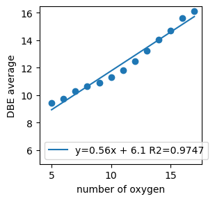
Using the obtained metrics, it is possible to classify samples by origin or property, train different models.