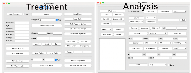
Graphical user interface of nomspectra

After installation nomspectra you can run GUI by the command:

python -m nomspectra

The GUI is pretty basic and not very flexible but it supports all basic operation.

The program’s capabilities are divided into two parts - treatment and analysis

Treatment

Download, view and save spectrum

You can upload a new spectrum without treatment, or a previously processed spectrum. To load a new spectrum, you need to select the new checkbox, and also fill the column separator that is used in the file, if the separator is tab - fill tab , comma as comma , etc., and also headers for m/z and intensity exactly the same as in the file. The file should not contain extra lines at the beginning and the end of the file - only the names of the columns and data.

After loading the spectrum, you can check what has loaded using the Print Spectrum button. If the columns are merged into one, then the wrong delimiter was probably used. Columns must include mass and intensity . You can also view the current spectrum at any other time the program is running.

If you open a file that has already been processed by this program, then, as usually, standard headers and a separator are used there, so it is not necessary to specify them.

When opening the spectrum, you can set limits on mass and intensity in the corresponding fields.

The spectrum can be saved Save Spectrum - a dialog box opens, the table is saved in text form. Also spectrum stored in buffer, so you can add it to analysis tab and operate on it.

Brutto formula generation and spectrum assignment

Range of elemetns is shown in list above elements and Isotopes fields.

By default, the following range of elements is used: C (from 4 to 50), O (from 0 to 25), H (4-100), N(0-3), S(0-2). To return to the standard selection press Reset .

If Rules bo is on (default) limits are also used for H/C (0.25-2.2), O/C (0-1), DBE-O<=10, and the nitrogen rule.

If you want to set a different set of elements and their range, then they need to be added one by one through the corresponding fields - Element, Isotope. If the element is the main one, then you can leave the Isotope field empty (for example, for carbon 12 - just fill in the element C), for specific isotopes fill in the appropriate fields (for example, C 13). Fill in the range Range from to. Press Add , the current set will be displayed.

For remove element click on row in list field and press remove button.

To generate brutto formulas, press Gen , the table will be displayed in the field below.

To assign formulas, enter the allowable error in the Err ppm field and maximum charge into Max Charge, chose mode (negative by default or positive) and press the Assign button.

After assigment you can remove peaks that don’t have 13C isotopes by C_13 button and also remove duplicates by dupl button.

You can load the background Load Background and remove it Remove Background. But for this it is necessary to use the background, to which formulas are also assigned - it should be processed in the same way as a spectrum and saved to a separate file.

TMDS generation

In some cases, the use of the mass difference statistics spectrum (TMDS) makes it possible to better carry out the procedure for assigning brutto formulas, to use smaller values ​​of the assignment error.

The elements for its generation are set in the same way as for the spectrum assignment. It makes sense to set negative starting values, such as -1, -4 for elements, since many differences involve negative values, such as C-1H4O.

Then you need to set the peak occurrence threshold in the mass difference spectrum, field P. The default value is 0.2, but with these conditions, sometimes about 1000 mass differences are generated and the subsequent assignment of the original spectrum takes a long time (5-15 minutes depending on the computing power of the computer)

You can try to use large values ​​depending on the number of mass differences (p=0.6, 0.7…), or limit the maximum number of formulas in TMDS - the N field.

By default, generation occurs only on the basis of peaks for which the presence of a peak with the C13 isotope is confirmed, but this restriction can also be removed - check C_13 if the spectrum is scarce initially and you want to generate more mass differences.

To generate TMDS, press Gen TMDS. It can be saved to a text file using the Save TMDS button.

After generating TMDS, you can use it and assign additional peaks in the spectrum using the Assign by TMDS button

Plotting spectrum and Van Krevelen diagrams in processing mode

To quickly check the correctness of the procedures being carried out, it makes sense to build the spectrum and the Van Krevelen diagram.

After loading the spectrum, you can plot the spectrum with the corresponding Plot Spectrum button. A new window will open, in which you can operate with the spectrum - select an area, zoom in, move, etc.

Van-Krevelen can be built with the appropriate button after assigning formulas. By default, forums containing sulfur and nitrogen will turn into colors (CHONS - red, CHOS - green, CHON - orange.

Recalibration

The spectrum can be recalibrated by different methods

• According to the standard. To do this, open the reference spectrum processed by the program Load Etalon, press Calc Recal by Etalon, the error progress will be displayed. After that, you can press recalibrate, after which the masses in the spectrum change, you need to reassign the formulas using Assign

• similarly, you can calculate recalibration by assignment error Calc Recal by Assign or by mass difference map Calc Recal by MDiff.

You can track the process by show assigning error - Show Assign Error

The error can be applied not to the entire range, but to a part, for this you need to fill in the range, press Range and Extrapolate. Once calculated error can be applied to other spectra - load Load Error or save Save Error to a file. You can upload your error table.

Analysis

Loading, saving, renaming spectra

Analysis can be performed only with spectra processed by this programm or by the nomspectra library; to work with other files, you need to bring the table headers in accordance with this library (‘mass’ as m/z, ‘intensity’ as Intensity, ‘,’ as separator)

You can load several spectra at once, to do this, click Multi Load and select files. Also you can add just treated spectrum with tab treatment by button Add_buffer

After uploading (may take some time), they will be displayed below in the field with names corresponding to the names of the files. If you need to rename or change it color or transparity onto diagram, then double click spectrum, enter a new parameters and press the OK button.

Also, if necessary, the spectrum can be removed from the collection - select spectrum by checkboxes and press the Remove button.

For Save spectra check them and click button Save. In this case, you will need to select a folder for saving, there it will create a folder out, where the spectra will be saved. Be careful, if such a folder already exists, the files will be overwritten if the names match.

Logical operations with spectra, Venn diagrams

Spectra can be added, subtracted, found in common, and similarity metrics can also be calculated. Select at last two spectrum.

The operation is performed for spectra that were selected by checkboxes. For substraction oder is matter, so place your spectra in desirabel oder by clicking it and moving it by buttuns up and down

After the operation is completed, the new spectrum will be appeared in the bottom of spectra list

• add. Addition of all spectra

• sub. Subtract all spectra from the first selected spectrum

• and. Select the formulas included in all spectra.

• xor. Formulas included in only one of all spectra.

• int_sub. Subtract all spectra from the first selected spectrum by intensity. Formulas whose intensity is higher in the other spectrum will be removed from the first one.

For plot venn diagramm of selected spectra click button venn. This operation can be done only for 2 or 3 spectra at once.

Calculation of parameters, normalization and cutting of spectra

Operations will be performed on selected spectra.

Calculate parameters - calculate. It may take some time, especially if there are many spectra. DBE, AI, NOSC and more will be calculated.

Spectral intensity can be normalized normalize by sum, maximum intensity, mean or median. Normalization will be carried out for each spectrum separately.

To display the generalized parameters of the spectra - select the method, by default mean weight - the intensity-weighted average parameters will be calculated. To display the results - press Count. You can also calculate similar parameters for a narrower section of the spectra - to do this, select the parameter intensity, mass…, how to cut >, <. = and fill in the field next. If the field is empty, cropping will not be performed.

Calculation results can be saved to csv file - SaveCSV

To crop the spectra, you need to select the cropping parameter - intensity, mass and more. Enter the number to cut into the field. If you need to truncate everything that is greater than this number, select >, if less than <. If you need to select only the given value, then =

Calculation of metrics, similarity matrix

Operations will be performed on selected spectra.

The intensity-weighted average distribution of formulas over molecular zones can be determined using the Classes button. A bar chart will be built (for ease of reading, it is worth stretching horizontally).

It is also possible to calculate the weighted average of the population intensity over the areas of the Van Krevelen diagram Squares. If you perform an operation on one spectrum, a population map will be displayed, if for few or all, a table will be displayed.

To plot the dependence of DBE on nO, press the button DBE vs nO. The linear section can be limited by fields nO

To calculate the similarity matrix, select a method and press Simmilarity, the thermal matrix will be displayed.

Output results can be saved to csv file - SaveCSV

Adjust image settings and save them

You can choose the resolution of generated images dpi and their relative size size.

To limit the ordinate, you need to enter two values ​​into the fields x1 and x2, for automatic adjustment, leave them empty. Similarly for the abscissa y1 y2.

To save the generated images, you need to select the folder for saving Path, and the image format. Click the Save checkbox. Pictures will be automatically saved in the selected folder.

Draw spectra, diagrams

Before draw except spectrum you should make calculate parameters - calculate

Selection of spectra. Adjustment of color, transparency

The colors for the spectra are automatically selected in the order:

[‘blue’,’red’,’green’,’orange’,’purple’,’brown’,’pink’,’gray’,’olive’,’cyan’]

If you want a specific color for the spectrum, then double click on it and correct it. The list of available colors can be found here: https://matplotlib.org/stable/gallery/color/named_colors.html Also for scatterplots, you can set the transparency value in the alpha field. By default it is 0.2, and when many spectra are selected, one by one may not be seen.

The order of their construction is determined by up to down. So if you want correct it click on spectra and move it button up and down.

Draw a mass spectrum

The usual mass spectrum can be plotted with the Spectrum button

Scatterplot for arbitrary parameters

Button Scatter selection of parameters - two fields to the right. The third field is responsible for how the size of the dots will be determined. The size of each point is defined as the ratio of a given parameter to its median in the entire spectrum. This value can be multiplied by an arbitrary number to increase or decrease the points - fill in the size field and also raise to a power - fill in the pow field. If you select the None parameter, then the size of the points will be the same and determined by the size field. Also you can plot combine scatter and density - ScatterDens

Distribution density

To build a one-dimensional distribution density - select the parameter of interest and press the button Density