Batch Processing

from nomspectra.spectrum import Spectrum
from nomspectra.spectra import SpectrumList
import nomspectra.draw as draw
import pandas as pd
import matplotlib.pyplot as plt
import os

Load spectra

We can load separate Spectrum, treat them and then join it in SpectrumList object which is a list of spectra

specs = SpectrumList()
for filename in sorted(os.listdir("data/similarity/")):
    if filename[-3:] != 'csv':
        continue
    spec = Spectrum.read_csv(f"data/similarity/{filename}", assign_mark=True)
    specs.append(spec)

specs.get_names()

['a_1', 'a_2', 'a_3', 'a_4', 'a_5', 'a_6']

Or directly load from folder if specs already treated

specs = SpectrumList.read_csv('data/similarity/')
specs.get_names()

['a_4', 'a_5', 'a_6', 'a_2', 'a_3', 'a_1']

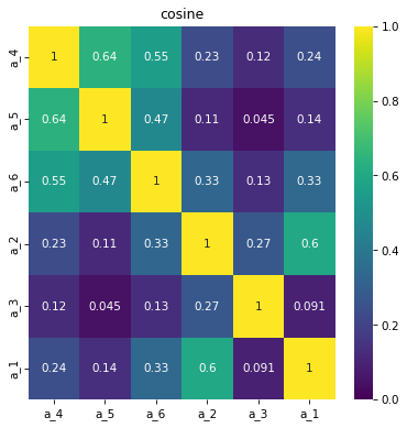
Calculate simmilarity index and plot matrix

Calculate simmilarity indexes. For now it common indexes - Cosine, Tanimoto and Jaccard

specs.get_simmilarity(mode='cosine')

array([[1.        , 0.63921734, 0.55387418, 0.22893115, 0.12221844,
        0.24206235],
       [0.63921734, 1.        , 0.46713676, 0.11426236, 0.04536192,
        0.13553428],
       [0.55387418, 0.46713676, 1.        , 0.3297159 , 0.12996979,
        0.33440804],
       [0.22893115, 0.11426236, 0.3297159 , 1.        , 0.27330141,
        0.59910651],
       [0.12221844, 0.04536192, 0.12996979, 0.27330141, 1.        ,
        0.0912144 ],
       [0.24206235, 0.13553428, 0.33440804, 0.59910651, 0.0912144 ,
        1.        ]])

And plot matrix

specs.draw_simmilarity(mode='cosine')

png

Calculate metrics

From spectra we can get molecular metrics

specs.get_mol_metrics()

	a_4	a_5	a_6	a_2	a_3	a_1
AI	-0.079344	-0.037731	-0.307631	0.444909	0.613860	0.171642
C	21.476279	21.143970	17.786572	22.186035	23.129087	17.967260
CAI	9.251700	8.712936	9.954005	15.300819	16.397214	12.064931
CRAM	0.552194	0.540266	0.485958	0.090364	0.035393	0.204550
DBE	12.644497	12.636119	8.106037	13.660797	16.722827	8.526630
DBE-O	0.806469	0.492241	0.560464	7.055005	10.396550	2.820194
DBE-OC	0.033105	0.017236	0.017788	0.298224	0.447654	0.118010
DBE_AI	0.419919	0.205085	0.273470	6.775581	9.990954	2.624301
H	20.004788	19.264393	21.578437	19.305284	15.211308	21.029147
H/C	0.941654	0.924041	1.220249	0.918817	0.655002	1.261374
N	0.341225	0.248690	0.217368	0.254807	0.398788	0.147887
NOSC	0.225485	0.268255	-0.290940	-0.289653	-0.039698	-0.601656
O	11.838028	12.143877	7.545574	6.605792	6.326276	5.706435
O/C	0.555214	0.575824	0.439298	0.295497	0.279618	0.315787
S	0.045326	0.038467	0.069625	0.024617	0.006808	0.048007
Unnamed: 0	5134.428335	1918.021934	1496.312157	841.325051	1782.231948	1584.499424
errorPPM	0.001824	0.029912	0.045206	-0.029267	-0.030579	0.000557
formula	NaN	NaN	NaN	NaN	NaN	NaN
mass	473.590881	472.240469	361.207872	395.774294	399.951346	331.795644
peakNo	5134.428335	1918.021934	1496.312157	841.325051	1782.231948	1584.499424
z	0.000000	0.000000	0.000000	0.000000	0.000000	0.000000

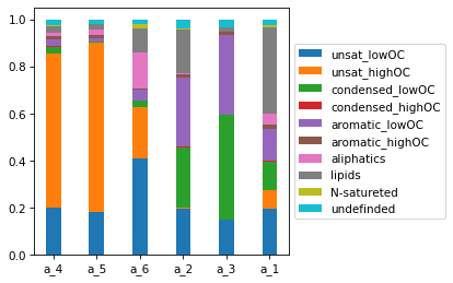
Get molecular class density and plot bar

specs.draw_mol_density()
specs.get_mol_density()

	a_4	a_5	a_6	a_2	a_3	a_1
unsat_lowOC	0.201447	0.183535	0.408356	0.195555	0.147491	0.196795
unsat_highOC	0.654447	0.716404	0.217642	0.006134	0.004349	0.080142
condensed_lowOC	0.026479	0.005946	0.028384	0.256306	0.441213	0.118184
condensed_highOC	0.002802	0.000989	0.000662	0.001651	0.002156	0.002919
aromatic_lowOC	0.028453	0.013982	0.044924	0.290728	0.336764	0.138210
aromatic_highOC	0.015343	0.011668	0.005026	0.014576	0.014677	0.016288
aliphatics	0.014729	0.023744	0.155616	0.005297	0.000097	0.045678
lipids	0.028270	0.022411	0.101287	0.186821	0.018383	0.369506
N-satureted	0.003950	0.000688	0.016474	0.005117	0.000000	0.006827
undefinded	0.024080	0.020633	0.021629	0.037814	0.034871	0.025451

png

Also we can calculate density of squares of Van Krevelen diagram

specs.get_square_vk()

	a_4	a_5	a_6	a_2	a_3	a_1
1	0.008942	0.004066	0.014149	0.046670	0.178541	0.009918
2	0.002034	0.001793	0.012627	0.033494	0.149713	0.005776
3	0.000819	0.000160	0.010486	0.046734	0.061893	0.010208
4	0.023089	0.017808	0.038597	0.041165	0.023237	0.069177
5	0.005045	0.003707	0.044065	0.153976	0.004767	0.293159
6	0.028251	0.009248	0.023760	0.356841	0.348926	0.188009
7	0.070833	0.049838	0.102810	0.199036	0.165541	0.093670
8	0.087435	0.083649	0.225485	0.060352	0.023909	0.103503
9	0.015644	0.021632	0.129569	0.008620	0.001865	0.045593
10	0.002791	0.006214	0.034856	0.006054	0.000000	0.027571
11	0.066727	0.092062	0.017016	0.035408	0.032921	0.039697
12	0.372026	0.420460	0.109793	0.010715	0.008141	0.040661
13	0.248249	0.219455	0.138720	0.000269	0.000090	0.048610
14	0.015856	0.013362	0.040365	0.000000	0.000000	0.011880
15	0.000423	0.001304	0.005874	0.000000	0.000000	0.001774
16	0.003531	0.008137	0.001184	0.000000	0.000211	0.002251
17	0.028628	0.036910	0.005151	0.000182	0.000000	0.003421
18	0.015810	0.010031	0.004591	0.000237	0.000123	0.003076
19	0.002573	0.000165	0.024572	0.000249	0.000000	0.001212
20	0.000423	0.000000	0.008698	0.000000	0.000000	0.000089

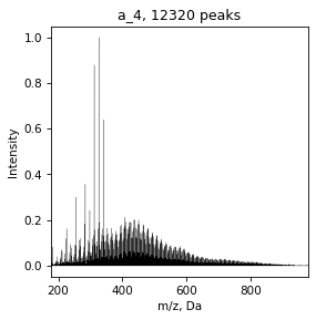
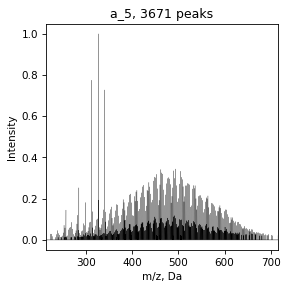
SpectrumList is a list

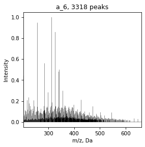
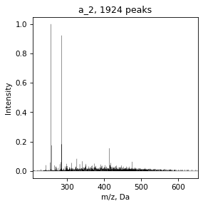
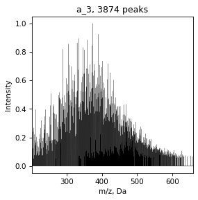
With SpectrumList object we can work as with list, for example, plot spectrum

for spec in specs:
    draw.spectrum(spec)

png

And save all data in folder

if 'temp' not in os.listdir():
    os.mkdir('temp')

specs.to_csv('temp')